halfBaked - RNA-seq - edgeR Differential Expression • halfBaked

Introduction

This is an example template for running a typical differential expression analysis using edgeR via halfBaked. It is meant to be a starting point for your own analysis and is not a comprehensive guide to all the options available in edgeR or halfBaked.

Load the Pin (or SummarizedExperiment)

This vignette assumes that you have already created a pin with the halfBaked package (see vignette("halfBaked Pin Generation Template")) that you want to load or that you have a SummarizedExperiment object that you want to use.

If you already have a SummarizedExperiment object, you can skip this step and load it directly.

library(halfBaked)
library(SummarizedExperiment)
library(pins)
library(openxlsx)
library(msigdbr)
library(BiocParallel)
library(rrvgo)

set.seed(7)

board <- board_url(params$board)
se <- pin_read(board, params$pin_name)

Dataset Description

If stored in the SummarizedExperiment, we can show the experiment description directly.

cat(metadata(se)$description)

Wang J. et al SciAdv 2020 - GSE135880 - Mouse OPCs with Eed KO - RNA-seq Data

This dataset contains O4+ immunopanned oligodendrocyte precursor cells (OPCs) from cortices of P5 or P6 Eed KO or control mice. See the associated publication for more details.

Please see the Pin generation code to view how this data was processed.

Run Differential Expression via edgeR

See halfBaked::get_edgeR_res() for more details on the parameters.

# To hold the results for each comparison.
res <- list()

# Whatever can be used as name of contrast vectors.
contrasts <- list(
    "Eed_cKO.v.Control" = c("Group", "Eed_cKO", "Control")
)

res <- get_edgeR_res(se,
    res.list = res, contrasts = contrasts,
)

# Cram DE results into SE metadata.
se.meta <- metadata(se)
se.meta$edgeR.Results <- res
metadata(se) <- se.meta

# Save all results to file if wanted.
dir.create("./de", showWarnings = FALSE)
write.xlsx(res, file = "./de/All.Comparisons.DEGs.edgeR.xlsx", overwrite = TRUE)

Enrichment/Over-representation Analyses

Hypergeometric enrichment analyses are pretty standard after differential expression. We use the run_enrichment() function to make these more convenient to run. This function largely uses the clusterProfiler package.

# Set species and database stuff for enrichments
if (params$species %in% c("human", "mouse")) {
    if (params$species == "human") {
        orgdb <- "org.Hs.eg.db"
        msig.species <- "Homo sapiens"
    } else {
        orgdb <- "org.Mm.eg.db"
        msig.species <- "Mus musculus"
    }
} else {
    stop("species parameter must be 'human' or 'mouse'")
}

# Edit if you'd like, don't recommend post-hoc LFC thresholding
sig_th <- 0.05
lfc_th <- 0
sig_col <- "FDR"
lfc_col <- "logFC"

kegg_res <- list()
rct_res <- list()
go_res <- list()

for (rez in names(res)) {
    df <- res[[rez]]$table

    bg <- df$ENSEMBL[!is.na(df[[sig_col]])]

    up_genes <- df$ENSEMBL[!is.na(df[[sig_col]]) &
        df[[sig_col]] < sig_th &
        df[[lfc_col]] > lfc_th]

    dn_genes <- df$ENSEMBL[!is.na(df[[sig_col]]) &
        df[[sig_col]] < sig_th &
        df[[lfc_col]] < -lfc_th]

    if (length(up_genes) > 0) {
        kegg_res <- run_enrichment(up_genes, bg,
            res.name = paste0(rez, "_up"),
            res.list = kegg_res, OrgDb = orgdb,
            method = "KEGG", species = params$species
        )

        rct_res <- run_enrichment(up_genes, bg,
            res.name = paste0(rez, "_up"),
            res.list = rct_res, OrgDb = orgdb,
            method = "Reactome", species = params$species
        )

        go_res <- run_enrichment(up_genes, bg,
            res.name = paste0(rez, "_up"),
            res.list = go_res, OrgDb = orgdb,
            method = "GO", species = params$species
        )
    }

    if (length(dn_genes) > 0) {
        kegg_res <- run_enrichment(dn_genes, bg,
            res.name = paste0(rez, "_dn"),
            res.list = kegg_res, OrgDb = orgdb,
            method = "KEGG", species = params$species
        )

        rct_res <- run_enrichment(dn_genes, bg,
            res.name = paste0(rez, "_dn"),
            res.list = rct_res, OrgDb = orgdb,
            method = "Reactome", species = params$species
        )

        go_res <- run_enrichment(dn_genes, bg,
            res.name = paste0(rez, "_dn"),
            res.list = go_res, OrgDb = orgdb,
            method = "GO", species = params$species
        )
    }
}

full_res <- c(kegg_res, rct_res, go_res)

Create Summary Table

Individual files are for the birds, I hate making supplemental tables.

dir.create("./enrichments_edgeR", showWarnings = FALSE)

# Excel sheets can only be 31 characters, so it is necessary to shorten the names
names(full_res) <- gsub("Reactome", "RCT", names(full_res))
names(full_res) <- gsub("Control", "Ctl", names(full_res))
names(full_res) <- gsub("\\.v\\.", "v", names(full_res))

write.xlsx(full_res, file = "./enrichments_edgeR/allresults.xlsx", overwrite = TRUE)

# Save to SE object.
metadata(se)$edgeR.enrichments <- full_res

Basic Visualization

A picture’s worth 10000 words of AI-generated slop.

my_theme <- theme(
    axis.text.y = element_text(size = 6, color = "black"),
    axis.text.x = element_text(color = "black"),
    axis.ticks = element_line(color = "black")
)

# Basic bar and dotplots for arbitrary top X enriched gene sets
for (comp in names(full_res)) {
    enr <- full_res[[comp]]
    message(comp)

    pdf(paste0("./enrichments_edgeR/", comp, "_Enrichments.Top30.pdf"),
        width = 6, height = 8
    )
    print(dotplot(enr, showCategory = 30, font.size = 7) + my_theme)
    print(dotplot(enr, size = "Count", showCategory = 30, font.size = 7) + my_theme)
    print(barplot(enr, showCategory = 30, font.size = 7) + my_theme)
    dev.off()

    # This collapses redundant GO terms into a single term based on similarity.
    # The set with the lowest p-value in each cluster is used as the label.
    if (grepl("GO", comp)) {
        enr <- simplify(enr)

        pdf(paste0("./enrichments_edgeR/", comp, "_collapsedEnrichments.Top30.pdf"),
            width = 6, height = 8
        )
        print(dotplot(enr, showCategory = 30, font.size = 7) + my_theme)
        print(dotplot(enr, size = "Count", showCategory = 30, font.size = 7) + my_theme)
        print(barplot(enr, showCategory = 30, font.size = 7) + my_theme)
        dev.off()
    }
}

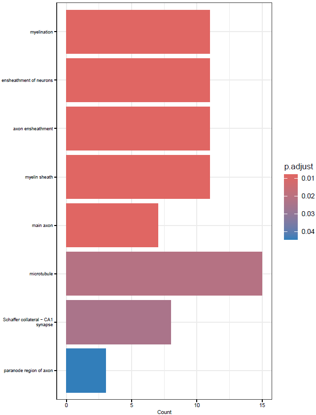
This will create simple dot and barplots like so:

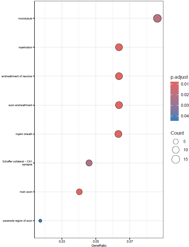
Clustering GO Terms

GO terms can be very redundant, which makes coming through the results and summarizing them a headache. One solution to this is to cluster terms with a high degree of overlap and then summarize the cluster.

onts <- c("BP", "CC", "MF")

up.col <- "#56B4E9"

gobp_res <- grep("GOBP", names(full_res))
gomf_res <- grep("GOMF", names(full_res))
gocc_res <- grep("GOCC", names(full_res))

clustered_res_size <- list()
clustered_res_uniqueness <- list()
clustered_res_log10_padjscore <- list()

for (ont in onts) {
    # Get the GO terms for the current ontology
    if (ont == "BP") {
        curr_go <- gobp_res
    } else if (ont == "CC") {
        curr_go <- gocc_res
    } else {
        curr_go <- gomf_res
    }

    godat <- GOSemSim::godata(orgdb, ont = ont)

    # Ignore these words, alter as wanted
    stoppers <- tm::stopwords(kind = "en")
    stoppers <- c(
        stoppers, "regulation", "positive",
        "negative", "process", "cell", "activity"
    )

    for (i in names(full_res)[curr_go]) {
        enr.up <- full_res[[i]]

        # Collapse similar terms, score by term size, uniqueness, or significance
        if (!is.null(enr.up)) {
            if (nrow(enr.up) > 2) {
                dir.create(file.path("enrichments_edgeR", "reduced"),
                    recursive = TRUE, showWarnings = FALSE
                )

                enr.up.sim <- calculateSimMatrix(enr.up$ID,
                    orgdb = orgdb,
                    ont = ont,
                    semdata = godat,
                    method = "Rel"
                )

                enr.up.scores <- -log10(enr.up$p.adjust)
                names(enr.up.scores) <- enr.up$ID

                enr.up.red.size <- reduceSimMatrix(enr.up.sim,
                    scores = "size",
                    threshold = 0.7, orgdb = orgdb
                )

                enr.up.red.unique <- reduceSimMatrix(enr.up.sim,
                    scores = "uniqueness",
                    threshold = 0.7, orgdb = orgdb
                )

                enr.up.red.score <- reduceSimMatrix(enr.up.sim,
                    scores = enr.up.scores,
                    threshold = 0.7, orgdb = orgdb
                )
                
                clustered_res_size[[i]] <- enr.up.red.size
                clustered_res_uniqueness[[i]] <- enr.up.red.unique
                clustered_res_log10_padjscore[[i]] <- enr.up.red.score

                write.table(enr.up.red.size,
                    file = file.path(
                        "./enrichments_edgeR/reduced",
                        paste0(i, ".termsim.Reduced.size.0.7.txt")
                    ),
                    sep = "\t",
                    row.names = FALSE, quote = FALSE
                )

                write.table(enr.up.red.unique,
                    file = file.path(
                        "./enrichments_edgeR/reduced",
                        paste0(i, ".termsim.Reduced.uniqueness.0.7.txt")
                    ),
                    sep = "\t",
                    row.names = FALSE, quote = FALSE
                )

                write.table(enr.up.red.score,
                    file = file.path(
                        "./enrichments_edgeR/reduced",
                        paste0(i, ".termsim.Reduced.log10_padjscore.0.7.txt")
                    ),
                    sep = "\t",
                    row.names = FALSE, quote = FALSE
                )

                pdf(
                    file.path(
                        "./enrichments_edgeR/reduced",
                        paste0(i, ".barplot.termsim.Reduced.size.0.7.pdf")
                    ),
                    width = 5, height = 6
                )
                p <- plot_clustered_terms_top(enr.up.red.size,
                    color = up.col,
                    n.top.terms = 5, xlabel = "term size", stoppers = stoppers
                )
                print(p)

                p <- plot_clustered_terms_top(enr.up.red.size,
                    color = up.col,
                    n.top.terms = 5, n.top.clusters = 20,
                    xlabel = "term size", stoppers = stoppers
                ) +
                    ggtitle("top 20 clusters by score")
                print(p)
                dev.off()

                pdf(
                    file.path(
                        "./enrichments_edgeR/reduced",
                        paste0(i, ".barplot.termsim.Reduced.uniqueness.0.7.pdf")
                    ),
                    width = 5, height = 6
                )
                p <- plot_clustered_terms_top(enr.up.red.unique,
                    color = up.col,
                    n.top.terms = 5, xlabel = "uniqueness", stoppers = stoppers
                )
                print(p)

                p <- plot_clustered_terms_top(enr.up.red.unique,
                    color = up.col,
                    n.top.terms = 5, n.top.clusters = 20,
                    xlabel = "uniqueness", stoppers = stoppers
                ) +
                    ggtitle("top 20 clusters by score")
                print(p)
                dev.off()

                pdf(
                    file.path(
                        "./enrichments_edgeR/reduced",
                        paste0(i, ".barplot.termsim.Reduced.log10padj_scores.0.7.pdf")
                    ),
                    width = 5, height = 6
                )
                p <- plot_clustered_terms_top(enr.up.red.score,
                    color = up.col,
                    n.top.terms = 5, xlabel = "-log10(adj.pval)", stoppers = stoppers
                )
                print(p)

                p <- plot_clustered_terms_top(enr.up.red.score,
                    color = up.col,
                    n.top.terms = 5, n.top.clusters = 20,
                    xlabel = "-log10(adj.pval)", stoppers = stoppers
                ) +
                    ggtitle("top 20 clusters by score")
                print(p)
                dev.off()
            }
        }
    }
}

# Again, tack onto SE
metadata(se)$edgeR.clustered_GO_enrichment <- list(
    size = clustered_res_size,
    uniqueness = clustered_res_uniqueness,
    log10_padjscore = clustered_res_log10_padjscore
)

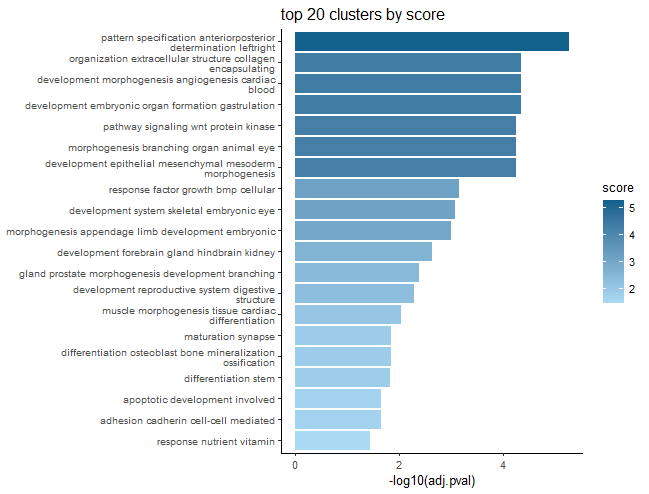
This will spit out barplots with the most frequent terms for each cluster as labels and the largest term size, uniqueness, or highest -log10(p-value) of a term as the representative score of the cluster.

The p-value scoring likely makes the most sense.

These plots are good for condensing many GO terms into clusters that can be meaningfully interpreted in a broad sense.

GSEA

Gene set enrichment analysis (GSEA) is another pretty typical follow-up to differential expression analyses.

Load Gene Sets

Our gene sets just need to be in a named list, where the name of each element corresponds to the gene set identifier and the element itself is just a vector of gene identifiers.

The MSigDB database is a very popular source of gene sets, as it contains numerous collections. We can use the msigdbr package for simple access to these gene sets.

In this case, we show how to create a nested list of lists, where the first level is the gene set collection/subcollection, and the second level are the named vectors with the actual gene set name and members.

# Set categories and subcategories that we want to retrieve, see msigdbr_collections()
# These vectors must be of equal length.
cats <- c("H", "C2", "C2", "C2", "C3", "C5", "C5", "C5", "C5", "C8")
subcats <- c(
    "", "CGP", "CP:KEGG", "CP:REACTOME", "TFT:GTRD",
    "GO:MF", "GO:BP", "GO:CC", "HPO", ""
)

msig_lists <- list()

# Get gene sets for each category and subcategory and stick in the msig.lists
for (i in seq_along(cats)) {
    cat <- cats[i]
    subcat <- subcats[i]

    msig <- msigdbr(species = msig.species, category = cat, subcategory = subcat)

    # Split into a named list
    msig_ls <- msig %>% split(x = .$gene_symbol, f = .$gs_name)

    # Stick in the list
    if (subcat == "") {
        outname <- cat
    } else {
        outname <- paste0(cat, "_", subcat)
    }

    msig_lists[[outname]] <- msig_ls
}

# We could also use custom gene sets, perhaps stored in a pin
# Potentially as nested lists for easier selection.
# board <- board_connect(server = params$board)
# gs <- pin_read(board, gs.pin)

Create Ranked Gene Lists

GSEA requires a ranked list of genes, so we will use the test statistic, as it is signed and correlates with both significance and effect size. The edgeR authors recommend using the p-value for ranking.

# Add as many comparisons as wanted here.
# Should match values in `names(dds.meta$DE.Results)`.
dges <- c("Eed_cKO.v.Control")

ranked_lists <- list()

for (d in dges) {
    out.res <- dds.meta$edgeR.Results[[d]]
    gsea.df <- out.res[!(is.na(out.res$padj)), ]

    gsea.df.gsea <- gsea.df$stat
    names(gsea.df.gsea) <- make.names(gsea.df$SYMBOL, unique = TRUE)

    ranked_lists[[d]] <- gsea.df.gsea
}

Run GSEA

Now we’re ready to perform GSEA for each of the ranked gene sets.

We’ll also loop through the gene collections to run on each individually.

See run_GSEA() for full parameters.

res_list <- list()

for (i in seq_along(ranked_lists)) {
    ranked_genes <- ranked_lists[[i]]
    ranked_name <- names(ranked_lists)[i]
    message(paste0("Running pre-ranked GSEA for: ", ranked_name))

    # Loop through the gene collections
    for (j in seq_along(msig_lists)) {
        msig_ls <- msig_lists[[j]]
        msig_name <- names(msig_lists)[j]

        # Remove the colon or it'll break file paths
        msig_name <- gsub(":", "_", msig_name)

        message(paste0("Using collection: ", msig_name))

        # Run GSEA
        res_list <- run_GSEA(msig_ls, ranked_genes,
            outdir = "./GSEA/", res.name = paste0(ranked_name, ".", msig_name),
            res.list = res_list
        )
    }
}

# Excel sheets can only be 31 chars, so it is often necessary to shorten the names
names(res_list) <- gsub("REACTOME", "RCT", names(res_list))

# Add to metadata of the SummarizedExperiment object
metadata(se)$DESeq2.GSEA <- res_list

Create Summary Table

The run_GSEA function generates a ton of output depending on how many ranked lists are used. Ultimately, it’s pretty nice to have that all in a single file for easy sharing/perusal, so we’ll write each results table to a worksheet of an excel file.

write.xlsx(res_list, file = "./GSEA/MSigDB.allresults.xlsx", overwrite = TRUE)
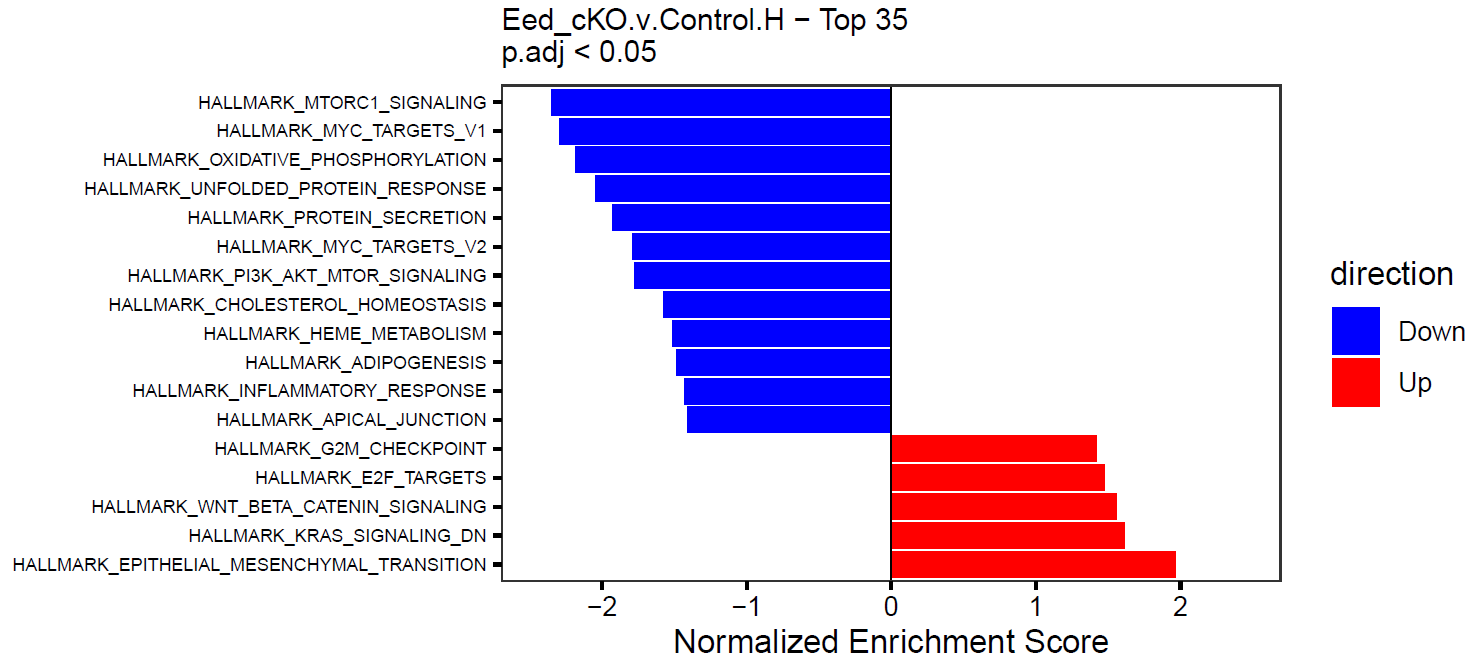
saveRDS(res_list, file = "./GSEA/MSigDB.allresults.RDS")

Create Summary Figures

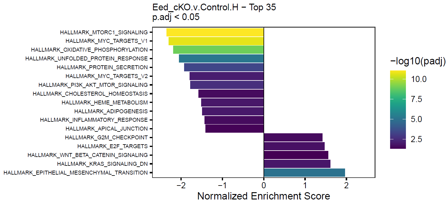
GSEA returns a lot of output and can be hard to summarize, so this is an attempt to make the results more compact by chucking the top X significant gene sets into a single figure.

We can do this for each element in our GSEA results list. See GSEA_barplot() for full parameters.

for (res in names(res_list)) {
    message(paste0("Plotting GSEA results for: ", res))

    p <- GSEA_barplot(
        gsea.res = res_list[[res]], genesets.name = res,
        padj.th = 0.05, top = 35
    )

    # Can also color by direction rather than adj. p
    p2 <- GSEA_barplot(
        gsea.res = res_list[[res]], genesets.name = res,
        padj.th = 0.05, top = 35, color.by.direction = TRUE
    )

    # Dynamic height adjustment
    h <- 2 + (0.07 * nrow(p$data))

    pdf(paste0("./GSEA/", res, ".GSEA_barplot.pdf"), height = h, width = 7)
    print(p)
    print(p2)
    dev.off()
}

This will create simple barplots like so:

Write Pin

The pin can now be saved with the new DE, enrichment, and GSEA data included.

# Write the pin with the new data
board <- board_connect(server = params$board)
pin_write(board, se,
    type = "rds", name = params$pin_name, title = params$pin_name,
    description = params$pin_description
)

# Can save the object locally if wanted as well.
saveRDS(se, file = "./se.RDS")

SessionInfo

Click to expand

## R version 4.5.1 (2025-06-13)
## Platform: x86_64-pc-linux-gnu
## Running under: Ubuntu 24.04.2 LTS
## 
## Matrix products: default
## BLAS:   /usr/lib/x86_64-linux-gnu/openblas-pthread/libblas.so.3 
## LAPACK: /usr/lib/x86_64-linux-gnu/openblas-pthread/libopenblasp-r0.3.26.so;  LAPACK version 3.12.0
## 
## locale:
##  [1] LC_CTYPE=C.UTF-8       LC_NUMERIC=C           LC_TIME=C.UTF-8       
##  [4] LC_COLLATE=C.UTF-8     LC_MONETARY=C.UTF-8    LC_MESSAGES=C.UTF-8   
##  [7] LC_PAPER=C.UTF-8       LC_NAME=C              LC_ADDRESS=C          
## [10] LC_TELEPHONE=C         LC_MEASUREMENT=C.UTF-8 LC_IDENTIFICATION=C   
## 
## time zone: UTC
## tzcode source: system (glibc)
## 
## attached base packages:
## [1] stats4    stats     graphics  grDevices utils     datasets  methods  
## [8] base     
## 
## other attached packages:
##  [1] rrvgo_1.20.0                BiocParallel_1.42.1        
##  [3] msigdbr_24.1.0              openxlsx_4.2.8             
##  [5] pins_1.4.1                  SummarizedExperiment_1.38.1
##  [7] Biobase_2.68.0              GenomicRanges_1.60.0       
##  [9] GenomeInfoDb_1.44.0         IRanges_2.42.0             
## [11] S4Vectors_0.46.0            BiocGenerics_0.54.0        
## [13] generics_0.1.4              MatrixGenerics_1.20.0      
## [15] matrixStats_1.5.0           halfBaked_0.99.0.9000      
## [17] BiocStyle_2.36.0           
## 
## loaded via a namespace (and not attached):
##   [1] splines_4.5.1               later_1.4.2                
##   [3] ggplotify_0.1.2             tibble_3.3.0               
##   [5] R.oo_1.27.1                 polyclip_1.10-7            
##   [7] graph_1.86.0                lifecycle_1.0.4            
##   [9] edgeR_4.6.2                 NLP_0.3-2                  
##  [11] lattice_0.22-7              MASS_7.3-65                
##  [13] SnowballC_0.7.1             magrittr_2.0.3             
##  [15] limma_3.64.1                sass_0.4.10                
##  [17] rmarkdown_2.29              jquerylib_0.1.4            
##  [19] yaml_2.3.10                 httpuv_1.6.16              
##  [21] ggtangle_0.0.6              askpass_1.2.1              
##  [23] zip_2.3.3                   reticulate_1.42.0          
##  [25] cowplot_1.1.3               DBI_1.2.3                  
##  [27] RColorBrewer_1.1-3          abind_1.4-8                
##  [29] purrr_1.0.4                 R.utils_2.13.0             
##  [31] ggraph_2.2.1                yulab.utils_0.2.0          
##  [33] tweenr_2.0.3                rappdirs_0.3.3             
##  [35] GenomeInfoDbData_1.2.14     enrichplot_1.28.2          
##  [37] tm_0.7-16                   ggrepel_0.9.6              
##  [39] tokenizers_0.3.0            tidytree_0.4.6             
##  [41] reactome.db_1.92.0          pheatmap_1.0.13            
##  [43] umap_0.2.10.0               RSpectra_0.16-2            
##  [45] pkgdown_2.1.3               codetools_0.2-20           
##  [47] DelayedArray_0.34.1         DOSE_4.2.0                 
##  [49] xml2_1.3.8                  ggforce_0.4.2              
##  [51] tidyselect_1.2.1            aplot_0.2.6                
##  [53] UCSC.utils_1.4.0            farver_2.1.2               
##  [55] viridis_0.6.5               jsonlite_2.0.0             
##  [57] tidygraph_1.3.1             ggridges_0.5.6             
##  [59] systemfonts_1.2.3           tools_4.5.1                
##  [61] treeio_1.32.0               ragg_1.4.0                 
##  [63] Rcpp_1.0.14                 glue_1.8.0                 
##  [65] gridExtra_2.3               SparseArray_1.8.0          
##  [67] xfun_0.52                   DESeq2_1.48.1              
##  [69] qvalue_2.40.0               dplyr_1.1.4                
##  [71] withr_3.0.2                 BiocManager_1.30.26        
##  [73] fastmap_1.2.0               openssl_2.3.3              
##  [75] digest_0.6.37               mime_0.13                  
##  [77] R6_2.6.1                    gridGraphics_0.5-1         
##  [79] textshaping_1.0.1           colorspace_2.1-1           
##  [81] GO.db_3.21.0                RSQLite_2.4.1              
##  [83] R.methodsS3_1.8.2           tidyr_1.3.1                
##  [85] data.table_1.17.6           graphlayouts_1.2.2         
##  [87] httr_1.4.7                  S4Arrays_1.8.1             
##  [89] graphite_1.54.0             pkgconfig_2.0.3            
##  [91] gtable_0.3.6                blob_1.2.4                 
##  [93] SingleCellExperiment_1.30.1 XVector_0.48.0             
##  [95] clusterProfiler_4.16.0      janeaustenr_1.0.0          
##  [97] htmltools_0.5.8.1           bookdown_0.43              
##  [99] fgsea_1.34.0                scales_1.4.0               
## [101] png_0.1-8                   wordcloud_2.6              
## [103] ggfun_0.1.8                 knitr_1.50                 
## [105] reshape2_1.4.4              nlme_3.1-168               
## [107] curl_6.3.0                  cachem_1.1.0               
## [109] stringr_1.5.1               parallel_4.5.1             
## [111] AnnotationDbi_1.70.0        treemap_2.4-4              
## [113] desc_1.4.3                  ReactomePA_1.52.0          
## [115] pillar_1.10.2               grid_4.5.1                 
## [117] vctrs_0.6.5                 slam_0.1-55                
## [119] promises_1.3.3              dittoSeq_1.20.0            
## [121] xtable_1.8-4                evaluate_1.0.3             
## [123] cli_3.6.5                   locfit_1.5-9.12            
## [125] compiler_4.5.1              rlang_1.1.6                
## [127] crayon_1.5.3                tidytext_0.4.2             
## [129] plyr_1.8.9                  fs_1.6.6                   
## [131] stringi_1.8.7               gridBase_0.4-7             
## [133] viridisLite_0.4.2           assertthat_0.2.1           
## [135] babelgene_22.9              Biostrings_2.76.0          
## [137] lazyeval_0.2.2              GOSemSim_2.34.0            
## [139] Matrix_1.7-3                patchwork_1.3.0            
## [141] bit64_4.6.0-1               ggplot2_3.5.2              
## [143] KEGGREST_1.48.0             statmod_1.5.0              
## [145] shiny_1.10.0                igraph_2.1.4               
## [147] memoise_2.0.1               bslib_0.9.0                
## [149] ggtree_3.16.0               fastmatch_1.1-6            
## [151] bit_4.6.0                   ape_5.8-1                  
## [153] gson_0.1.0

halfBaked - RNA-seq - edgeR Differential Expression

Jared Andrews

18 June 2025

Introduction

Load the Pin (or SummarizedExperiment)

Dataset Description

Run Differential Expression via edgeR

Enrichment/Over-representation Analyses

Create Summary Table

Basic Visualization

Clustering GO Terms

GSEA

Load Gene Sets

Create Ranked Gene Lists

Run GSEA

Create Summary Table

Create Summary Figures

Write Pin

SessionInfo